Summary of wav2vec 2.0 Research Paper
Introduction Humanity speaks in about 7111 distinct languages. As amazing as it might seem that our species can communicate in so many ways, it presents a colossal challenge in terms of creating good quality speech recognition systems. The challenge ensues from the fact that the neural networks demand large amounts of labeled data, which is hard to come by for a majority of these languages. The languages that do not have large amounts of data sets for training AI models are called low-resource languages.
The wav2vec 2.0 model [1] enables the creation of speech recognition technology for the aforementioned low-resource languages by providing a self-supervision style framework that learns from unlabeled training data. The wav2vec 2.0 is the latest iteration of wav2vec models, the earlier ones being vq-wav2vec [2] (from which it derives some inspiration) and wav2vec [3] (the version 1 of wav2vec). The self-supervised learning approach has gained some prominence over the years, where the practice is to learn data representations from unlabeled samples followed by the fine-tuning of the model on labeled data.
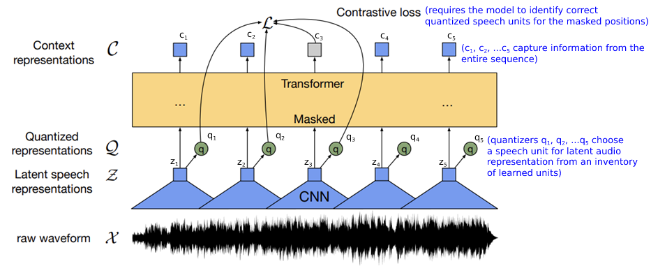
This paper presents such a self-supervised learning framework that pretrains a model on more accessible unlabeled audio data followed by fine-tuning on a targeted dataset. It processes the raw waveform of the audio using a CNN to get the latent audio representations. These representations are then fed to a Quantizer and a Transformer. The following figure describes the different states of activities described above to give a visual sense, with first state being the CNNs receiving the audio signal as:

followed by the representations from CNN being fed to the Transformer and the Quantizers (represented as green circles in the figure Fig. 2 below):
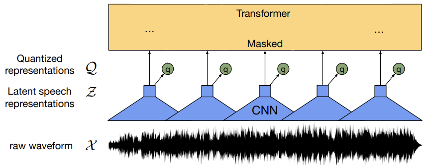
A quantizer converts values from a continuous space into a finite set of values in a discrete space.
This quantizer chooses a speech unit, which could be an independent clause or subclausal unit, for the latent audio
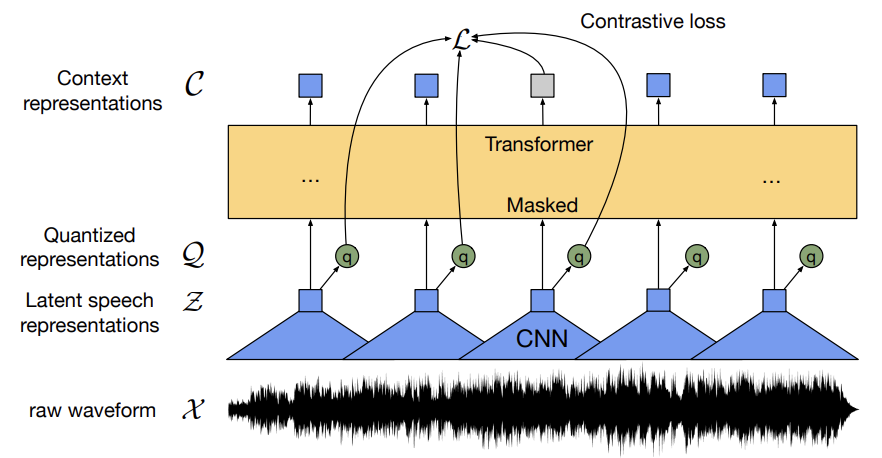
representation from a store of learned speech units. Approximately 50% of the audio representations are masked before
being fed into the transformer. The transformer adds information from the entire audio sequence. Finally, the output of
the transformer is used to solve a contrastive task. This task requires the model to identify the correct quantized speech
units for the masked positions.
The authors of this Paper then propose that the discrete speech units be learnt through a Gumbel-Softmax distribution [4] thus enabling the backward pass through the Quantization module and aiding the joint learning of the discrete speech units alongside the contextualized representations.
After the pre-training, the authors fine-tuned the model for speech recognition with a
Connectionist Temporal Classification loss [5], by adding a linear projection on top of the context network to predict a word token at each timestep.
To put everything mentioned above in the context, wav2vec 2.0 provides a framework for pre-training on unlabeled data followed by fine-tuning on a smaller labeled dataset. In the pre-training stage, about 50% masked input is fed to a Transformer (shown in the dark yellow block in Fig 3 above) that outputs a sequence of vectors, which tries to reconstruct the masked input. Transformers being quite computing resource intensive, typically using square the length of each signal, can’t be fed the audio signal directly as it has a lot of samples. Hence, the workaround is to down-sample using convolution neural networks (shown in blue in Fig. 3 above) that would summarise each window of the speech signal. The contrastive loss function (marked as in Fig. 3 above) uses a cosine similarity check on the quantized output of the CNN serving as the ground truth and the Transformer output, which is a sequence of vectors and identify the correct quantized unit from the incorrect ones (referred to as distractors in the Paper).
ModelThe wav2vec 2.0’s architecture and pre-training process have 4 major elements: feature encoder, quantization module, masking, and context network.
Feature EncoderIt is a 7-layer, (single-dimensional) - convolutional neural network with 512 channels at each layer. It takes in a raw input waveform that is normalized to zero mean and unit variance. Its objective is to reduce the dimension of the audio signal, by converting raw waveform into a sequence of feature vectors every 20 milliseconds.
The above transformation is expressed in the paper as \(\cal{f:X \mapsto Z}\), where \(\cal{X}\) represents the raw input audio signal and \(\cal{Z}\) being the output, with the latent speech representations \(\cal{z}_1\)\(\cal{, z}_2\)\(\cal{,...}\)\(\cal{, z}_T\) for \(\cal{T}\) time-steps.
The raw waveform is normalized before being sent to the CNN, followed by a Layer Normalization, and a GELU activation function. GELU is an abbreviated form of Gaussian Error Linear Unit. The GELU nonlinearity weights inputs by their percentile, rather than gates inputs by their sign as in ReLUs, making them smoother than ReLU.
A schematic of the feature encoder can be visualised as:
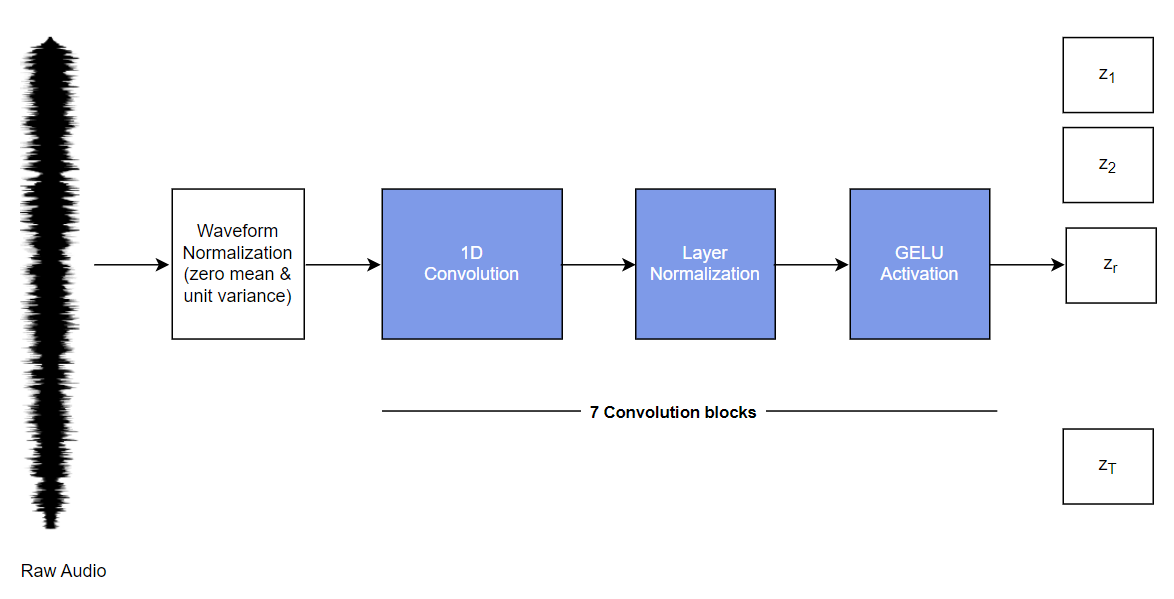
Following are the details of the 7 convolution blocks shown in the figure Fig. 4, above.
| Block Number | 1 | 2 | 3 | 4 | 5 | 6 | 7 |
| Kernel Width | 10 | 3 | 3 | 3 | 3 | 2 | 2 |
| Stride | 5 | 2 | 2 | 2 | 2 | 2 | 2 |
| Channel Size | 512 | 512 | 512 | 512 | 512 | 512 | 512 |
Based on data from Table 1, the kernel width and strides of the convolutional layers decrease with increasing block numbers, which can be read as the network depth. Also, feature encoder has a total receptive field of 400 samples that is equal to 25 milliseconds of audio data encoded at a sample rate of 16 kHz.
Quantization module A critical issue of using a Transformer for speech processing is the continuous nature of speech. While written language provides the natural capability for discretisation into words or sub-words, hence creating a finite vocabulary of discrete units, speech doesn’t have similar sub-units. Though phones could be used to discretise, it would necessitate a completely labeled dataset, making the approach unwieldy to be pre-trained on unlabeled data.
To facilitate this discretization of latent \(\cal{z}\) vectors to a finite set of speech representations, the Paper uses a technique called Product Quantization [6], which is a type of vector quantizer, that can decompose a high-dimensional vector space into a cartesian product of subspaces and then quantize these subspaces separately. It is a scope reduction technique, and not a dimensionality reduction one. In this technique, vectors are mapped from a large vector space to a finite number
of regions in that space. Each vector in these finite regions is called a code vector or a codeword. and the set of all the codewords is called a codebook.
In this Paper, there are \(\text{2}\) groups (denoted by \(\textit{G}\)) of latent variables in the codebook and \(\text{320}\) latent variables (denoted by \(\textit{V}\)) in each group of
the codebook. So, there are \(\text{2}\) groups (\(\textit{G}\)) with \(\text{320}\) possible entries (\(\textit{V}\)) in each group (\(\textit{G}\)). As mentioned in the preceding paragraph, a
Product Quantization is implemented using cartesian product of all the iterables items provided as the argument (implemented using itertools.product(*iterables)),
which in this case would be \(\text{2}\) lists with \(\text{320}\) entries, and hence there can be a theoretical maximum of \(\text{320}\times\text{320}=\text{102,400}\) speech units.
The input to the quantization module are a set of latent representation vectors \(\cal{z}_1\)\(\cal{, z}_2\)\(\cal{,...}\)\(\cal{, z}_T\) and the output is a set of quantization vectors \(\cal{q}_1\)\(\cal{, q}_2\)\(\cal{,...}\)\(\cal{, q}_T\).
In order to construct the output quantization vectors \(\cal{q}_1\)\(\cal{, q}_2\)\(\cal{,...}\)\(\cal{, q}_T\), the algorithm iterates over the Codebooks, \(\text{G(=2)}\) and in each iteration, selects an entry, \(\textit{e}\)) from the matrix \(\Bbb{R}^{\text{V}\times\text{d/G}}\) using Gumbel Softmax (described in the next paragraph), ending up with (\(\text{G}\)) vectors (\(\textit{e}_1\)\(\textit{, e}_2\)\(\textit{,...}\)\(\textit{, e}_G\)), each having size \(\text{d/G}\), which are concatenated, hence giving a vector in \(\Bbb{R}^\text{d}\) and then to get vector \(\cal{q}\), this vector in \(\Bbb{R}^\text{d}\) is multiplied with a quantization projection matrix to give an \(\text{f-dimensional}\) vector, mathematically expressed as a linear transformation \(\Bbb{R}^\text{d}\mapsto\Bbb{R}^\text{f}\) to obtain a quantization vector \(\cal{q}\in\Bbb{R}^\text{f}\) space.
The \(\cal{z}_1\)\(\cal{, z}_2\)\(\cal{,...}\)\(\cal{, z}_T\) are multiplied by a Quantization matrix, and turned into Logits (\(\cal{l}\))), i.e., \(\cal{z}\mapsto\cal{l}\), where
\(\cal{l}\in\Bbb{R}^{\text{G}\times\text{V}}\) space, and the choice of \(\text{G}\) and \(\text{V}\) will be derived from Gumbel softmax given by the following expression

The \(\textit{p}_{g, v}\) above is the probability of choosing the \(\textit{v-th}\) codebook entry for group \(\textit{g}\); \(\textit{n} = -\text{log}(-\text{log}(\textit{u}))\) is the Gumbel noise. A Gumbel noise is a sample (\(\textit{u}\)) from uniform (\(\cal{U}\)(\(\text{0, 1}\))), i.e., \(\textit{u}\) ~ \(\cal{U}\)(\(\text{0, 1}\)), and then perform \(-\text{log}(-\text{log}(\textit{u}))\) on it. The reason to use natural logarithms is due to the exponential terms in the expression in Fig. 5 above. The \(\tau\) (tau) is the temperature, the bigger the value of \(\tau\), the smoother the distribution.
A major benefit of using Gumbel Softmax is that it enables the backpropagation by making the
choice of Codebook entries above to be continuous rather than discrete, and hence fully differentiable. So, the target variables (\(\cal{q}\)) are also updated as part of the backpropagation, which is again quite a unique strategy.
So, for the forward pass the choice of an entry \(\textit{e}_j\) in (\(\textit{e}_1\)\(\textit{, e}_2\)\(\textit{,...}\)\(\textit{, e}_G\)) would be an \(\text{argmax}_j\textit{p}_{g,j}\) (the \(\text{argmax}_j\textit{p}_{g,j}\) is not differentiable). For the backward pass, where the differentiability is necessary, the framework is approximating the choice of entry using the Gumbel Softmax, that is going to provide the true gradient of the Gumbel Softmax outputs, which makes it differentiable.
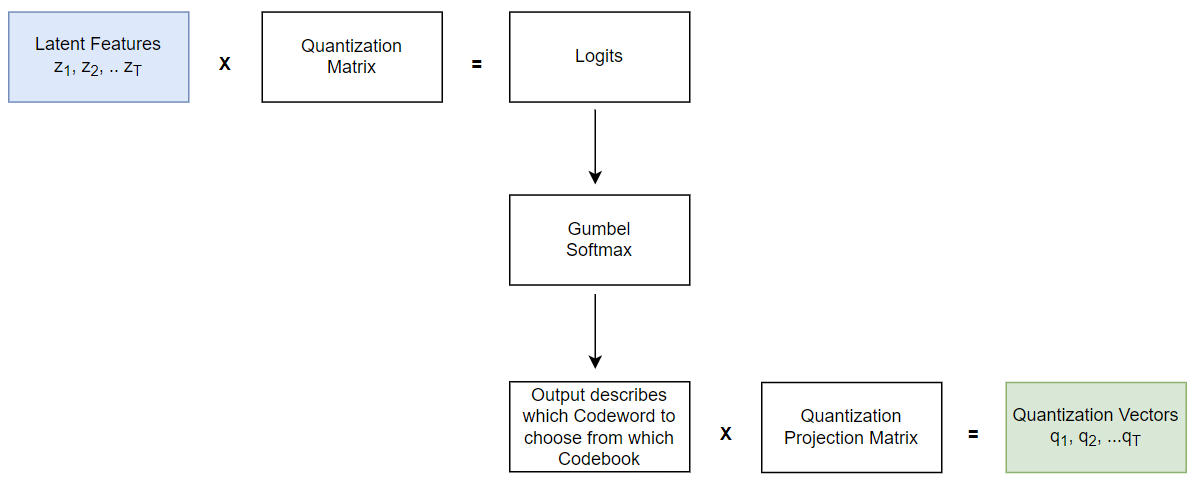
To summarise, latent features learnt from the CNN are multiplied by a quantization matrix in order to get the logits, which is a score for each of the possible entries \(\textit{V}\)) (or Codewords) in each group \(\textit{G}\)) (or Codebook). A Gumbel Softmax samples one entry \(\textit{V}\)) from each \(\textit{G}\)), after converting these logits into probabilities, and the operation is fully differentiable in the backward pass. A temperature argument (\(\tau\) in the expression shown in Fig. 5) introduces a small randomness effect.
To better visualise the above explanation, a schematic of the Quantization module showing an overview of different operations and steps of
functionalities involved is shown below.
MaskingA proportion of the feature encoder outputs are Masked before being fed to the Transformer. A certain proportion "\(\textit{p}\)" of the sequence of the latent speech representation output from the feature encoder are randomly selected to become the starting indices and then subsequent "\(\textit{M}\)" consecutive time steps from every such sampled index are masked. These "\(\textit{M}\)" consecutive time-steps are referred to as "\(\textit{span}\)" and since the starting points are randomly sampled, these spans can overlap.
In the Paper, a value of \(\textit{p}=\text{0.065}\) and \(\textit{M}=\text{10}\) time-steps were chosen, that produced approximately \(\text{49}\%\) masking of the time steps.
For illustration, if \(\textit{p}=\text{2}\) and \(\textit{M}=\text{6}\), then the schematic with overlapping spans would look like the following:
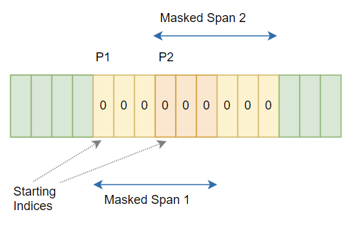
The computed masking indices (using \(\textit{p}=\text{0.065}\) and \(\textit{M}=\text{10}\)) are assigned a value of \(\textit{0}\) in the code. Consequently, the system is trained to predict the speech units that are masked, which is the purpose of Masking in this framework. This scheme draws its influence from Masked-Language Modeling of BERT (Bidirectional Encoder Representations from Transformers).
Contextualized representations with TransformersA core element of the wav2vec 2.0 framework is the Transformer [7] encoder. Transformer model’s origin could be tied to the necessity of language translation use cases in NLP. It has an encoder-decoder architecture, however, various two other types of Transformers also exist, that are encoder-only and decoder-only. The Transformer type used in wav2vec 2.0 is encoder-only type.
A Transformer’s encoder has many stacked encoder layers, where each one of the encoder blocks receive a sequence of positional embeddings and feeds them through the sub-layers. The first of these blocks is a multi-head self-attention block comprising of a number of parallel self-attention layers followed by a fully connected feed-forward layer applied to each input embedding. An attention mechanism is the core idea in Transformer networks. It helps the encoder to focus on the input tokens that are most relevant at each time step. This enables the encoder to understand the contextual information (i.e., connections between different input tokens in a sequence). The Transformer in this Paper uses a multi-head self-attention blocks. Each head calculates a scaled dot product using queries, keys, and values as inputs. The attention is calculated using \(\text{softmax}(\textit{QK}^T/\sqrt{d}_k)\textit{V}\), where \(\textit{Q}\) = query matrix, \(\textit{K}\) = key matrix, and \(\textit{V}\) = value matrix. The resultant of each scaled dot product attention operation is concatenated to form a matrix which
retains the context information for each positional embedding. Following screenshots provide a visualisation of the above.
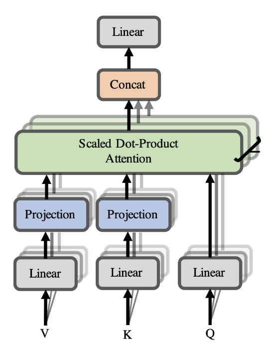
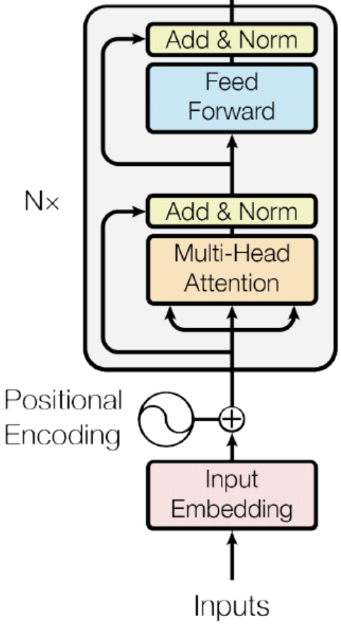
The set of output vectors from Feature Encoder \(\cal{z}_1\)\(\cal{, z}_2\)\(\cal{,...}\)\(\cal{, z}_T\) are fed to the Transformer, mathematically expressed as \(\cal{g:Z \mapsto C}\), where \(\cal{Z}\) represents the latent speech representations mentioned above as \(\cal{z}_1\)\(\cal{, z}_2\)\(\cal{,...}\)\(\cal{, z}_T\) and \(\cal{C}\) being the representations capturing information from the entire sequence \(\cal{c}_1\)\(\cal{, c}_2\)\(\cal{,...}\)\(\cal{, c}_T\).
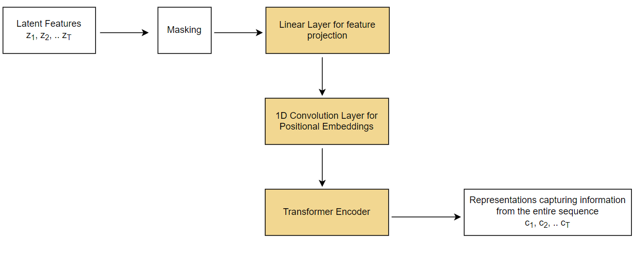
There are 2 versions of wav2vec 2.0 model – BASE and LARGE. For the BASE version of the model, the input latent feature vectors \(\cal{z}_1\)\(\cal{, z}_2\)\(\cal{,...}\)\(\cal{, z}_T\) are processed through 12 Transformer blocks, whereas for the LARGE version, they are processed through 24 blocks. Since, the latent feature vectors have a dimension of 512, they need to be transformed to match the Transformer encoder’s dimension of \(\text{768}\) for BASE and \(\text{1024}\) for LARGE. A linear layer for feature projection is used for this transformation so that output of Feature encoder can match with the inner dimension of the Transformer encoder.
Since, the output of the Feature Encoder even after creating representations from audio signal tend to be quite long, it is quite difficult to perform positional encoding in the absolute sense, so relative positions are considered, which is the difference between two absolute positions. One way to implement this strategy could be, to have a convolution with a long kernel size as the first layer of the Transformer, which is going to deliver the relative positions. So, instead of fixed positional embeddings which encode absolute positional information, a convolution layer is used that acts as a relative positional embedding.
Following is a schematic of the context network part of the model, that uses a Transformer encoder.
TrainingThe wav2vec 2.0 Paper specifies a two-step training process: Pre-training and Fine-tuning. The Pre-training step trains the wav2vec 2.0 model to help it form parameters using self-supervised learning on unlabeled data that can be used in speech recognition related tasks. The fine-tuning stage transfers the captured knowledge in the form of weights (formed during the pre-training step) to target tasks with small amount of labeled data.
Pre-trainingWhen this Paper came out the trend with Language models or Natural Language Processing was doing pre-training followed by fine-tuning on downstream tasks. This Paper introduced a similar paradigm into the arena of speech, along with using Transformers, which were quite rampant in Computer vision and NLP during the time, into Speech.
The Pre-training step is about learning from unlabeled data, i.e., learning from speech, like a child first learns to listen and then learns to speak, read, and write. This Paper introduced learning representations by listening only, quite like what a human would do.
However, since raw audio has a lot of samples, feeding all of it to a Transformer-based model wouldn’t have been wise, as Transformers don’t come cheap, and its cost would be the length of the signal-squared, and would be so to process every signal.
To get around that the first step is to down-sample using 7 convolution blocks. The derived latent speech representation is sent along 2 different paths:
- 1. For Quantization, where these quantized representations serve as the ground truth.
- 2. For masking, which is followed by a Linear layer, a convolutional positional embedding and then to a Transformer Encoder which provide the context representations.
A schematic of the Pre-Training process is shown below (Fig. 11). All the green-shaded
boxes represent networks having learnable weights.
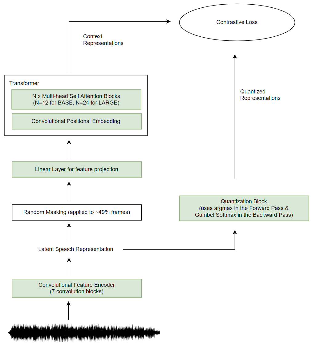
As listed above, the model randomly masks about \(\text{49}\%\) frames of the latent speech representation and feeds it to the Transformer (through other layers as mentioned above in Point 2 and shown in Fig. 11), which then reconstructs these masked parts.
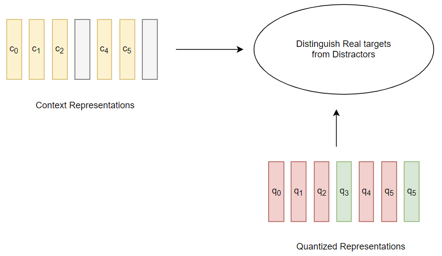
The Contrastive loss function then evaluates the cosine similarity between these reconstructed representations and the matched quantized representation. While the contrastive loss needs to identify the true quantized latent speech representation amongst a set of candidates (containing both the real one and distractors), another loss called Diversity loss function encourages these quantized units to be as diverse as possible through use of equal entries in each of the Groups of
Codebook while choosing members in the group which become the quantized ground truth units by maximizing the entropy of the averaged softmax distribution. This allows the quantized units to be as different from each other as possible.
The objective function, which is a sum of Contrastive and Diversity losses, encourages the Transformer to reconstruct masked parts accurately.
This step is like the masked language model task in BERT. A schematic of the mechanics of contrastive loss described above is shown in the following figure.
BackpropagationAs part of the minimizing the contrastive loss, the backpropagation would go all the way back to update the weights in the Convolutional Feature Encoder (the \(\text{1}^{st}\) block after the raw audio file in the Fig. 11). Besides this backpropagation path, there is another path which goes back through the Quantization block (enabled by the Gumbel Softmax in the Backward Pass shown in Fig. 11). In this backpropagation path, it would update the model for performing Quantization.
So, while the Transformer is ultimately trained using the Contrastive loss as the objective function, and as a result makes all the parameters better, but also makes the Quantization better.
This is how the wav2vec 2.0 framework described in the Paper jointly learns contextualized speech representations and an inventory of discretized speech units.
Ablations using continuous & quantized, inputs & targetsThere are a few ablations performed in the Paper, with different combination of strategies for using continuous/quantized context network inputs and continuous/quantized targets. The results shown below is a screenshot taken from the Paper, which shows that continuous inputs with
quantized targets performed best followed by continuous inputs with continuous targets.

Contrastive LossA contrastive task is used to train on unlabeled speech data in the pre-training process. The framework masks a proportion of the feature encoder outputs, or time steps before feeding them to the context network. However, inputs to the quantization module are not masked.
Masking is defined using two hyper-parameters "\(\textit{p}\)" and "\(\textit{M}\)". The framework masks the latent speech representation output of feature encoder \(\cal{z}_1\)\(\cal{, z}_2\)\(\cal{,...}\)\(\cal{, z}_T\) by randomly sampling a certain proportion \(\textit{p}\) of all time steps to be starting indices and then mask the subsequent \(\textit{M}\) consecutive time steps from every sampled index, without replacement.
A value of \(\textit{p}=\text{0.065}\) and \(\textit{M}=\text{10}\) time-steps produced approximately \(\text{49}\%\) of all time steps to be masked in the Paper.
Now, for a masked latent representation \(\cal{z}_T\), the framework would have a context representation \(\cal{c}_T\) such that it is able to predict the correct quantized representation
\(\cal{q}_T\) amongst a set of other quantized representations. To understand this in the context of Fig. 3, (again copied below for the ease of reference) which shows arrows to the contrastive
loss from the Transformer output and Quantization outputs.
in the context of this example
Let us consider the above Copy of Fig. 3, especially the arrows emerging out of the Quantized representations marked "\(\text{q}\)" in green circles and the arrow emerging from the grey
output node of the Transformer. In order to construct a coherent speech clause on the fly, the framework looks at some portions of the speech from the 3 quantization nodes shown in the
diagram as \(\text{q}_1\), \(\text{q}_2\), and \(\text{q}_3\), and one of the portions amongst these 3 options, i.e., \(\text{q}_3\) is going to give the correct choice and other 2
(\(\text{q}_1\) and \(\text{q}_2\)) would be incorrect. Now, there exists a
discrete choice between these 3 options. The problem is to identify the quantized latent speech representation for a masked time step \(\text{c}_3\) within a set of distractors \(\text{q}_1\) and \(\text{q}_2\).
The diversity loss described in the next section would strive to make \(\text{q}_1\), \(\text{q}_2\), and \(\text{q}_3\) as diverse choices as possible so that the contrastive loss can actually find a good contrast
amongst the choices \(\text{q}_1\), \(\text{q}_2\), and \(\text{q}_3\). The contrastive loss is given by the following expression.

To address the issue of identifying the correct choice of \(\text{q}\) in the example, consider the vector output of Transformer \(\text{c}_t\) and quantization output \(\text{q}_t\). The cosine similarity between these two is to be scored.
The cosine similarity is given by the following expression

Now, there would be 3 scores, since there are 3 quantization output nodes considered in this example above. The idea is to be able to increase the probability of \(\text{c}_t\) being very similar to \(\text{q}_t\), the true masked one (shown in the numerator of the contrastive loss in Fig. 14) and decrease the similarity with other two distractors (shown in the denominator of the contrastive loss in Fig. 14).
To summarise the above, the model compares the cosine similarity between the projected context vector \(\text{c}_t\) and the correct positive target \(\text{q}_t\) along with all negative distractors \(\text{q}\). The contrastive loss favors higher cosine similarity scores with the correct positive target and penalizes higher cosine similarity scores with distractors.
Diversity LossBesides the contrastive loss described above, there is one other issue here of the diversity of the choices while choosing \(\textit{e}_j\) in (\(\textit{e}_1\)\(\textit{, e}_2\)\(\textit{,...}\)\(\textit{, e}_G\)) using Gumbel Softmax. To re-state, the algorithm iterated over the Codebook, \(\textit{G}\) and in each iteration, selected an entry, \(\textit{e}\) from the matrix \(\Bbb{R}^{\text{V}\times\text{d/G}}\) using Gumbel Softmax and the question is whether these choices are as diverse as possible.
The diversity loss expression shown below facilitates the maximisation of the entropy of the
Gumbel-Softmax distribution, by preventing the model to always choose from a small sub-group of codebook entries.

Objective Function
The diversity loss is added to pre-training loss to encourage the model to more frequently utilise all the codebook entries more equally and is shown by the expression below.

Fine-tuningThe authors have skipped doing quantization during this stage of training, while retaining masking. A randomly initialized linear projection layer is added on top of the context representation. The Paper mentions a modified version of SpecAugment being applied to the signal, which is then fed to Feature Extractor followed by the Transformer that produces the contextualized representations, followed by a Linear layer that classifies these representations to their corresponding token class.
The model then is fine-tuned with CTC (Connectionist Temporal Classification) loss. CTC is a way to get around not knowing the alignment between the input and the output and is particularly useful in this use case, as an alignment between sequences is needed, but that alignment is difficult to locate.
A schematic diagram for the fine-tuning step is shown below, followed by a detailed description of the Connection Temporal Classification technique in the later section.
Please scroll further down to view the schematic diagram of the fine-tuning step.
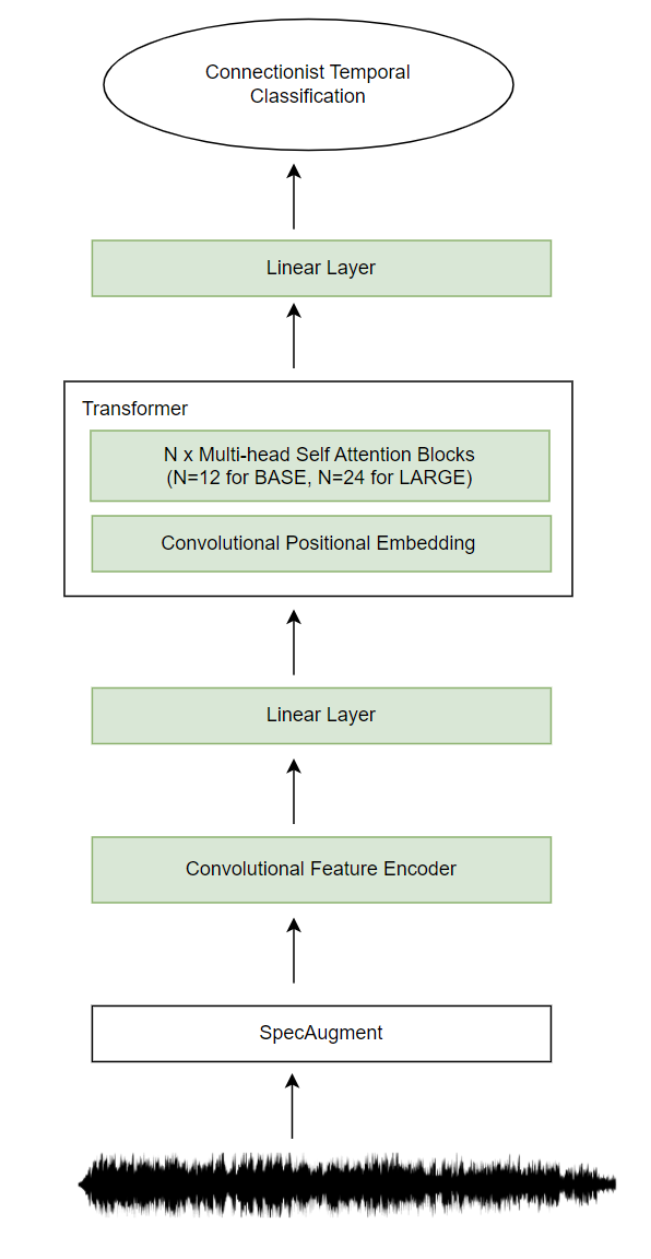
learnable weights
Connectionist Temporal Classification (CTC)It is a way to get around not knowing the alignment between the input and the output. In supervised speech recognition tasks, where given a dataset of audio clips and corresponding transcripts, it is hard to know how the characters in the transcript align to the audio, thus making training a speech recognizer particularly hard. Specifically, 3 such scenarios could exist:
- 1. Both input audio and output transcript can have different lengths.
- 2. The ratio of the lengths of input audio and output transcript can vary.
- 3. There may not be a correspondence of the elements (accurate alignment) of input audio and output transcript.
The CTC algorithm overcomes these challenges by collapsing repeating characters not separated by blank. For a given audio input it gives us an output distribution over all possible text transcript outputs. This distribution can be used to either infer a likely output or to assess the probability of a given output.
The CTC algorithm can assign a probability for any output given an audio input. The key to computing this probability is how CTC thinks about alignments between inputs and outputs. The CTC algorithm is alignment-free, i.e., it doesn’t require an alignment between the input and the output. However, to get the probability of an output given an input, CTC works by summing over the probability of all possible alignments between the two. The CTC alignments give us a natural way to go from probabilities at each time-step to the probability of an output sequence.
Pre-training experiments in the Paper The Paper lists 2 quite “infrastructure-heavy” experiments where the model configurations use the same encoder architecture but differ in the Transformer setup:
- 1. BASE contains 12 transformer blocks, model dimension 768, inner dimension (FFN) 3,072 and 8 attention heads. Batches are built by cropping 250k audio samples, or 15.6sec, from each example. Crops are batched together to not exceed 1.4m samples per GPU and trained on a total of 64 “V100” GPUs for 1.6 days; the total batch size is 1.6h.
- 2. LARGE model contains 24 transformer blocks with model dimension 1,024, inner dimension 4,096 and 16 attention heads. Authors cropped 320k audio samples, or 20sec, with a limit of 1.2m samples per GPU and train on 128 “V100” GPUs over 2.3 days for Librispeech and 5.2 days for LibriVox; the total batch size is 2.7h.
Conclusions drawn The main goal of the proposed framework of wav2vec 2.0 in this Paper [1] is to learn powerful representations from speech audio alone to create a pre-trained model that can be fine-tuned for speech recognition. The experiments in the paper have clearly shown a large potential of pre-training on unlabeled data for speech processing: when using only 10 minutes of labeled training data, or 48 recordings of 12.5 seconds on average, the authors have achieved a WER of 4.8/8.2 on test-clean/other of Librispeech. The model results are a state of the art on the full Librispeech benchmark for noisy speech. On the clean 100-hour Librispeech setup, wav2vec 2.0 outperformed the previous best result while using 100 times less labeled data.
So, wav2vec 2.0 model learns basic speech units used to tackle a self-supervised task. It is
trained to predict the correct speech unit for masked parts of the audio, while at the same time learning what the speech units should be, thus opening the doors to perform speech recognition in low-resource languages where transcribed audio data is very difficult to come by.
References
- [1] Alexei Baevski, Henry Zhou, Abdelrahman Mohamed, and Michael Auli. 2020. wav2vec 2.0: A Framework for Self-Supervised Learning of Speech Representations. arXiv. DOI:https://doi.org/10.48550/ARXIV.2006.11477
- [2] Alexei Baevski, Steffen Schneider, and Michael Auli. 2019. vq-wav2vec: Self-Supervised Learning of Discrete Speech Representations. arXiv. DOI:https://doi.org/10.48550/ARXIV.1910.05453/li>
- [3] Steffen Schneider, Alexei Baevski, Ronan Collobert, and Michael Auli. 2019. wav2vec: Unsupervised Pre-training for Speech Recognition. arXiv. DOI:https://doi.org/10.48550/ARXIV.1904.05862
- [4] Eric Jang, Shixiang Gu, and Ben Poole. 2016. Categorical Reparameterization with Gumbel-Softmax. arXiv. DOI:https://doi.org/10.48550/ARXIV.1611.01144
- [5] Alex Graves, Santiago Fernández, Faustino Gomez, and Jürgen Schmidhuber. 2006. Connectionist Temporal Classification: Labelling Unsegmented Sequence Data with Recurrent Neural Networks. In Proceedings of the 23rd International Conference on Machine Learning (ICML ’06), Association for Computing Machinery, Pittsburgh, Pennsylvania, USA, 369–376. DOI:https://doi.org/10.1145/1143844.1143891
- [6] Hervé Jégou, Matthijs Douze, and Cordelia Schmid. 2011. Product Quantization for Nearest Neighbor Search. IEEE transactions on pattern analysis and machine intelligence 33, (January 2011), 117–28. DOI:https://doi.org/10.1109/TPAMI.2010.57
- [7] Ashish Vaswani, Noam Shazeer, Niki Parmar, Jakob Uszkoreit, Llion Jones, Aidan N. Gomez, Lukasz Kaiser, and Illia Polosukhin. 2017. Attention Is All You Need. arXiv. DOI:https://doi.org/10.48550/ARXIV.1706.03762